What is Time and Space Complexity

There’s a reason companies ask questions about data structures and algorithms during interviews, because while almost anyone can code, not all think like a programmer.

Independent of programming language, interesting to learn and important to understand concepts in Software Engineering is time and space complexity. You have to think about them before writing any unit of code where speed or space is critical, and even talk about (especially in the case of an interview) after writing it.

Let’s go through the very basics of time and space complexity, what it is, why we care, how to measure and what the purpose of all of it really is.

By the time we are done, every other questions you might have can be explained with a reply to your comment, so feel free to drop your thoughts, questions and contributions in the comments section below.

What is Time and Space Complexity?

Let’s take a step back and talk about just the basics of time and space complexity.

The efficiency of every algorithm or function you have written in the past or going to write can be measured in terms of their time and space complexities expressed in Big Omega or Big O notation.

Big O notation is a mathematical notation that describes the limiting behavior of a function when the argument tends towards a particular value or infinity.

What is Space Complexity?

Put simply, space complexity is the total amount of additional memory space used by an algorithm or program.

Assuming we had to traverse an array in our program, two important approaches used to achieve that in programming are iteration and recursion.

What Is Time Complexity?

It is the number of steps that a program takes in terms of the size of input.

Basically, how long an algorithm takes to complete.

We will create a simple scenario to demonstrate what time complexity is.

For instance, let’s say an algorithm is giving an array of floating-point numbers to it sum up.

As an iterator starts at zero and goes up through the size of the input, we do something inbetween, in this case, add the current value to a total values’ variable, and finally return the total.

All of these are steps that each takes a certain amount of time.

In this case, the time complexity will then be, given this size of input of its length, how many steps this program took.

If the input array size is 10, one at a time, it will take ten journeys or iterations.

How to Calculate The Complexity of an Algorithm

Calculating the complexity of an algorithm involves analyzing how the algorithm’s performance (time or space) scales with the input size. Two common types of complexity are time complexity and space complexity. Here’s a guide on how to calculate them:

Time Complexity:

1. Count Basic Operations:

• Identify the basic operations performed in your algorithm. These could be assignments, comparisons, arithmetic operations, or any significant steps.

1. Express Operations in Terms of Input Size:

• Represent the number of basic operations in terms of the input size n. For example, if you iterate through an array, express the number of iterations as n.

1. Eliminate Constants and Less Dominant Terms:

• Focus on the most dominant term(s) and eliminate constants. For example, if you have an expression like “3n^2 + 2n + 5,” the time complexity is O(n^2) because the quadratic term dominates as n approaches infinity.

1. Determine the Overall Time Complexity:

• Sum up the complexities of individual steps. If you have nested loops or recursive calls, multiply the complexities. The overall time complexity is the highest order of the dominant term.

Space Complexity:

1. Identify Memory Usage:

• Identify the additional memory used by your algorithm. This includes variables, data structures, and any other memory allocations.

1. Express Space Usage in Terms of Input Size:

• Represent the amount of memory used in terms of the input size n. If you have an array of size n, it contributes O(n) space.

1. Eliminate Constants and Less Dominant Terms:

• Similar to time complexity, focus on the most dominant term(s), eliminate constants, and express the space complexity in big O notation.

1. Determine the Overall Space Complexity:

• Sum up the space complexities of individual components. If there are recursive calls or nested structures, add up or multiply the complexities. The overall space complexity is the highest order of the dominant term.

Tips:

• Worst-case vs. Average-case vs. Best-case:
• Consider different scenarios. Typically, you focus on the worst-case scenario when analyzing algorithm complexity, but it’s valuable to understand average and best cases too.
• Iterative vs. Recursive:
• When dealing with recursive algorithms, use recurrence relations to express the time complexity. It often involves solving equations to find closed-form solutions.
• Amortized Analysis:
• For some algorithms with varying time complexities, amortized analysis helps calculate the average cost over a sequence of operations.
• Benchmarking and Profiling:
• Sometimes, practical testing and profiling are essential to understand the real-world performance of an algorithm.

Most Common Time and Space Complexities and Their Meanings:

Time Complexities

1. Constant Time Complexity (O(1)):
   
   This is like grabbing something from your backpack. No matter how full it is, finding that item takes the same quick amount of time – constant!
2. Logarithmic Time Complexity (O(log n)):
   
   Think of a magical book where each page helps you eliminate half of the remaining options. It’s efficient and gets the job done faster as you go – logarithmic!
3. Linear Time Complexity (O(n)):
   
   Imagine making a sandwich. The more ingredients you have, the more time it takes, but it’s a straightforward process – linear!
4. Linearithmic Time Complexity (O(n log n)):
   
   Picture sorting a deck of cards by dividing it into smaller piles, sorting them, and then combining. It’s quicker than sorting the whole deck at once – linearithmic!
5. Quadratic Time Complexity (O(n^2)):
   
   If you have a to-do list and, for each task, you create a sublist of things to do, it takes a bit more time as the list grows – quadratic!
6. Cubic Time Complexity (O(n^3)):
   
   This is like adding another layer of detail to your to-do list for every task. It works well for small lists but can get slow for bigger ones – cubic!
7. Exponential Time Complexity (O(2^n)):
   
   Imagine a tree growing exponentially. It’s powerful for small tasks but becomes a bit much as things get bigger – exponential!
8. Factorial Time Complexity (O(n!)):
   
   If you’re arranging things in all possible ways, like planning a party, the time it takes grows astronomically – factorial!
9. Polynomial Time Complexity (O(n^k)):
   
   This is like a mix of quadratic, cubic, or any other polynomial growth. The ‘k’ is the degree of complexity – polynomial!
10. Amortized Time Complexity:
    It’s like looking at the average time spent over a series of activities. It helps smooth out occasional high-cost operations.

Space Complexities:

11. Constant Space Complexity (O(1)):
    
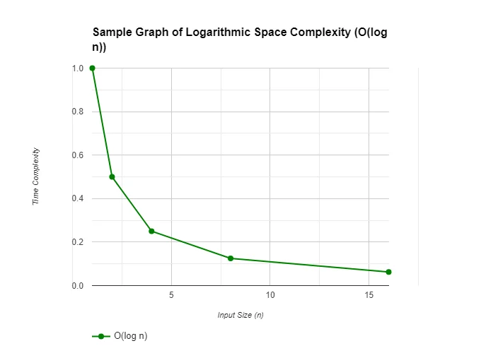
    Just like having a fixed-size backpack, regardless of how much stuff you’re carrying – constant space!
12. Logarithmic Space Complexity (O(log n)):
    
    Similar to logarithmic time, it’s about using memory more efficiently as the input size grows – logarithmic space!
13. Linear Space Complexity (O(n)):
    
    Memory usage grows in a linear fashion with the input size, just like your backpack getting a bit fuller – linear space!
14. Quasilinear Space Complexity (O(n log n)):
    
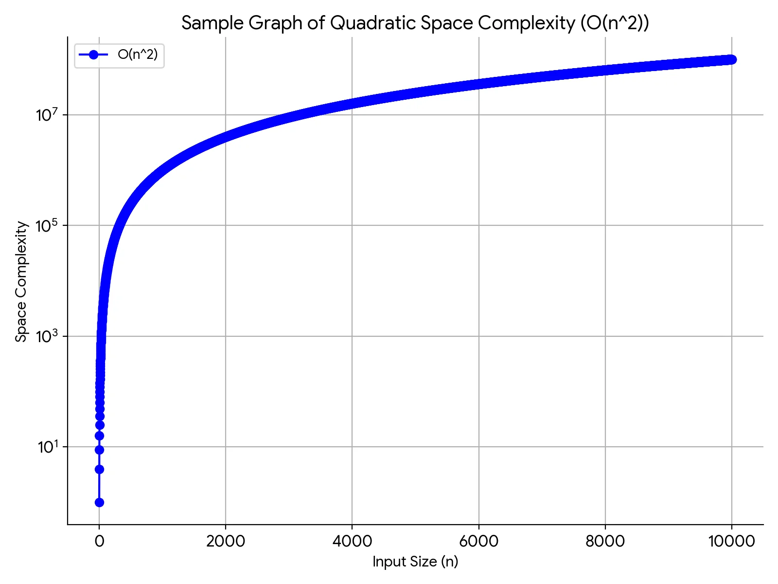
    It’s like a mix of linear and logarithmic space – common in algorithms with linearithmic time complexity.
15. Quadratic Space Complexity (O(n^2)):
    
    If you have a to-do list, and for each task, you create a sublist of things to remember or store additional information, it takes up more memory as the list grows – quadratic! Each task’s sublist contributes to the overall space used, and the memory requirements grow quadratically with the size of the list.
16. Cubic Space Complexity (O(n^3)):
    
    This is like adding another layer of detailed information to your to-do list for every task, and each sublist may have sublists of its own. It works well for small lists but can lead to significant memory usage for larger ones – cubic! The memory requirements increase cubically with the size of the list, making it less efficient for handling larger datasets.
17. Polynomial Space Complexity (O(n^k)):
    
    Memory grows polynomially with the input size, depending on the degree ‘k’ – polynomial space!
18. Exponential Space Complexity (O(2^n)):
    
    Memory usage grows exponentially with the input size, much like the time complexity – exponential space!
19. Factorial Space Complexity (O(n!)):
    
    Similar to factorial time complexity, memory needs explode as you consider all possible arrangements – factorial space!
20. Auxiliary Space Complexity:
    It’s the extra memory required during algorithm execution, not counting the initial input space.

Conclusion

Some people find Big O scary but it’s really not. The underlying concepts are not particularly hard to understand.

In summary, we use Big O notation to describe the performance of an algorithm and this helps to determine if a given algorithm is scalable or not which basically means is this algorithm going to scale well as the input grows really large.

So just because your code executes quickly on your computer doesn’t mean it’s going to perform well when given large data set.

Get practical today, join me as we solve even the hardest of LeetCode problems like they were nothing.